As instructors, we are deeply familiar with the frequentist approach to statistics—a powerful framework built on long-run frequencies, p-values, and the “reject” or “fail to reject” dichotomy. But what if we could directly address the questions our students (and we ourselves) often want to ask: “How likely is my hypothesis, given the data I’ve collected?” or “How should I update my beliefs in the face of new evidence?”
Now it’s time to learn the fundamentals of Bayesian logic and learn key terms so you can “speak Bayes.”
This module provides an intuitive, example-driven introduction to the Bayesian mindset. It’s a rational way to approach decision-making that allows us to move beyond binary outcomes and think in terms of distributions of belief. We will explore how to formally combine prior knowledge with new data to arrive at a more refined understanding of the world.
Learning Objectives
Upon completion of this module, you will be able to:
Define the core components of Bayes' Theorem: the prior, likelihood, posterior, and marginal likelihood.
Differentiate between the Bayesian (degree of belief) and frequentist (long-run frequency) interpretations of probability.
Apply Bayes' Theorem to solve a practical diagnostic problem.
Analyze real-world scenarios and marketing claims through a Bayesian lens.
Explain how personal beliefs and uncertainty can be represented as probability distributions.
Describe how Bayesian updating allows different initial beliefs to converge as more data is collected.
This is often suggested to be an image of Thomas Bayes, but is probably not him (Bellhouse, 2004). Included as a "teachable moment." Now enjoy seeing it reposted on a thousand blogs knowing this. One of the paid "Learn Bayes" sites even features it heavily as their logo. Oops!
A painting of Pierre Simon Laplace.
A Note on History
If Bayes’ theorem predated frequentist methods, why didn’t Bayes become the standard? Bayesian approaches can be computationally intensive, and until just the past few decades was not really feasible for most people. But don’t worry; we’ve got computers to do that for us now!
1. The Core Idea: Bayes’ Theorem
The concept is credited to Thomas Bayes, a Presbyterian minister in the 1700s, but it was later independently described and popularized by Pierre Simon Laplace. I would show you a picture of Bayes, but the only image we have that purportedly depicts Bayes is questionable at best (see Bellhouse, 2004). I don’t want to perpetuate misinformation, but include it here as a “teachable moment.” Despite this, the image has been reposted on a hundred blogs. However, we do have paintings of Laplace, and he was an interesting character in his own right. He is also responsible for formalizing the “Law of Error” that forms the backbone of frequentist tests many of us are more familiar with (e.g., t-tests). It’s slightly off topic for us right now, but I encourage you to read a bit about Laplace if you get a chance.
As we discovered in Module 1, Bayesian thinking is focused on Beliefs. Decision-making requires you to have an internal model of the world, and you want to make sure you are constantly updating that model of the world to make it as accurate as possible. You take your existing beliefs, or Prior, combine that with Data you observe in the world, compare the likelihood of that data under your prior beliefs, and update the beliefs to account for the new information.
So what did Bayes actually come up with? He came up with a conditional probability formula that basically shows how to figure out the relationships between your expectations and the data you observe so you can update your beliefs accordingly. Fair warning, this is going to look “math-y” for a second but bear with me, we’re about to explain each of these pieces. In terms of complexity, we’re just adding, multiplying, and dividing small numbers. The formula is mostly made up of labels for the concepts you’ve already learned, so don’t let the labels intimidate you.
Note on Symbols
The symbol | means “given.” So when you read something like P(H | D) it should be read as “the probability of the hypothesis given the data.”
Bayes’ Theorem
Bayes Theorem takes the form of a formula:
P(H | D) = P(D | H) * P(H) / P(D)
Where
P(H | D) - The Posterior: The probability of the hypothesis H being true given the observed data D. This is the updated belief we want to compute.
P(D | H) - The Likelihood: The probability of observing the data D, given that the hypothesis H is true. This quantifies how well the hypothesis explains the data.
P(H) - The Prior: The initial belief about the probability of the hypothesis H before seeing the data. This is based on previous knowledge or assumptions.
P(D) - The Marginal Likelihood: The total probability of observing the data D under all possible hypotheses. Its main job is to scale the result into a valid probability between 0 and 1.
From this, we can assess a few things. First and most obviously, we can combine our existing beliefs (Prior) with new information (Data) to update our beliefs about the world. You might notice if your prior is already similar to the data, the posterior value doesn’t change much. This makes sense because the data aren’t surprising given what you already know, so you don’t need to adjust your internal model much. Another thing to notice is that your prior beliefs influence your posterior beliefs. This captures the idea that two people observing the same evidence may not get to the same conclusion – but the data should move them both in the same direction. The third thing to notice for now is that it doesn’t matter how much data we collect; rather, we can adjust our beliefs even if we only have a small amount of data; if we get more later we can just update again. You simply rinse and repeat this process; your old posterior likelihood becomes your new prior likelihood for the next round.
It turns out that this framework is incredibly powerful for creating accurate models of the world. This has been influential in fields like information theory to help explain how streams of information can be processed over time, which in turn helps us understand naturally intelligent systems like the brain, and inspires us to make streamlined artificial systems.
Bayesian Updating Calculator
An interactive tool to understand Bayes' Theorem.
Bayes' Theorem
P(A|B) = [P(B|A) * P(A)] / P(B)
P(A|B) - Posterior: The updated probability of A after considering B.
P(B|A) - Likelihood: The probability of B, given that A is true.
P(A) - Prior: Your initial belief in the probability of A.
P(B) - Marginal: The overall probability of observing B.
10.0%
90.0%
20.0%
Calculating...
Change in Belief
Explore the Relationships
Strong Evidence, Weak Belief
Set the Prior to be very low (e.g., 1%). Now, imagine you get strong evidence: set Likelihood high (95%) and Marginal low (5%). See how much the Posterior jumps? Strong, rare evidence can dramatically change your mind.
Weak Evidence, Strong Belief
Start with a very high Prior (e.g., 90%). Now, get some contradictory evidence by setting the Likelihood low (e.g., 20%). Notice that your final belief doesn't drop that much. A strong initial belief is hard to change.
The "Surprise" Factor
Set Prior and Likelihood to 50%. Now, slide the Marginal from high to low. When the evidence is common (high Marginal), it doesn't change your belief much. When it's rare (low Marginal), it has a huge impact on your final belief!
An Important Distinction: Likelihoods versus Probabilities.
You’re probably used to probabilities. If I flip a standard coin 1000 times, you’d expect it to come up heads about 500 times. Probabilities look forward. They start with a known model or hypothesis (e.g., “this coin is fair, so P(Heads) = 0.5”) and predict the chances of seeing various future outcomes.
Probability asks: “If I know the rules of the game, what’s the chance of a certain event happening?” “If I flip a fair coin three times, what is the chance of getting 3 heads?”
Likelihoods, on the other hand, look backward. They start with the data you’ve already collected and evaluate how plausible your model or hypothesis is, given that data. You’re not calculating the chance of the event happening; you’re assessing how well a specific hypothesis explains the event that already happened.
Likelihood asks: “Now that I’ve seen an event happen, how likely is it that the rules of the game I was assuming are the correct ones?” “If I flip heads three times, how likely is it that the coin is fair?”
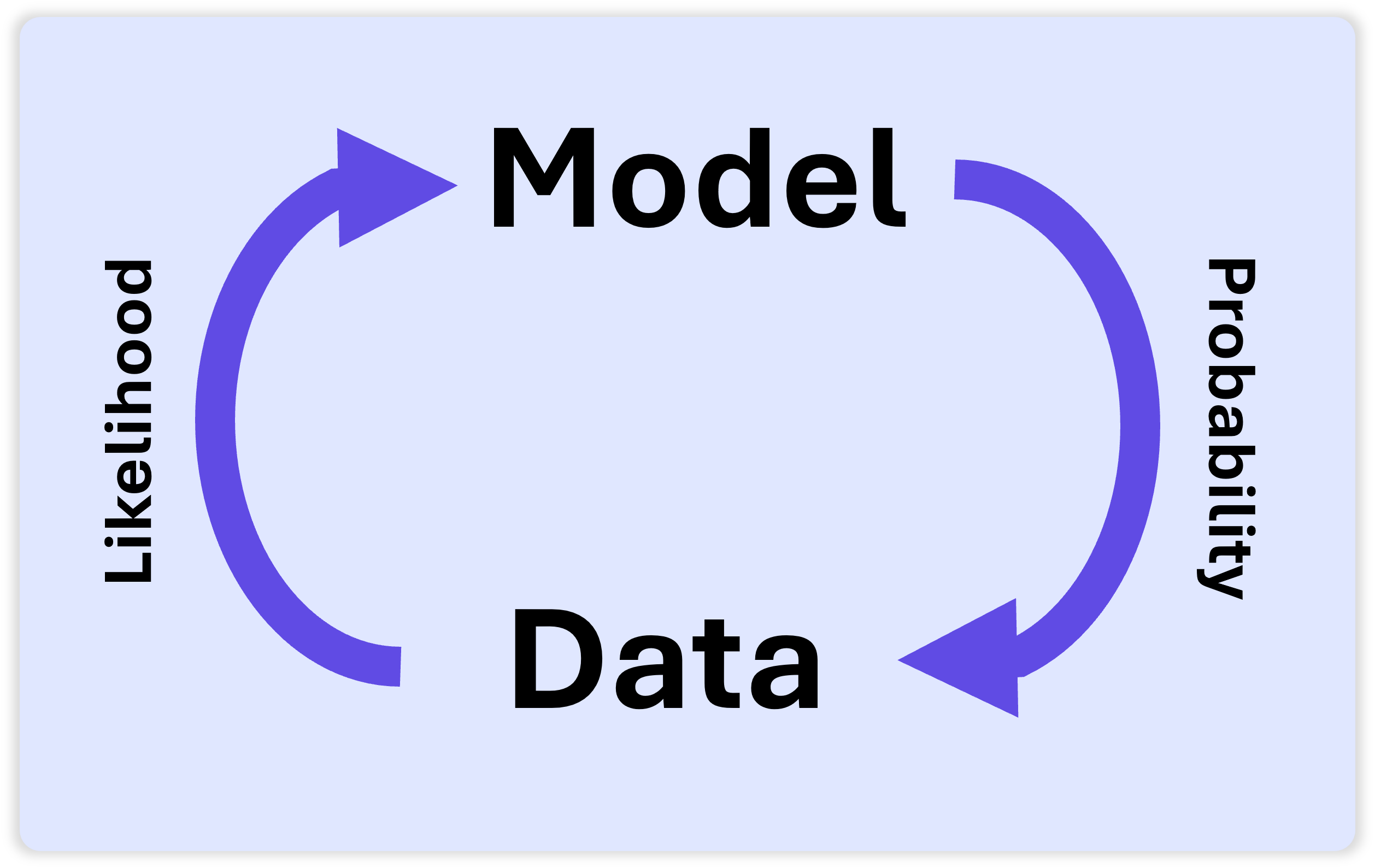
The Prediction Loop
The loop between using a model to predict events, and the observed events to improve the model. Probability lets you predict events using your model, and likelihood lets you see how well your model fit the data.
Likelihoods let you go back and check your models of the world. Were they a good fit? If not, you can adjust them for the future. You can have several models you are testing at once, directly comparing their likelihoods. Imagine that you had two hypotheses you wanted to compare. You could calculate how well the data fit one model, then the other, and directly compare how much better (if at all) one model fit the data over the other.
In fact, this is exactly what a Bayesian hypothesis test aims to do: Create a “null” model and an “alternative,” and then compare: which one matches the data better? This is called a Bayes Factor, and we’ll see more about that in the Bayesian t-test module later on.
Because you can include multiple likelihoods at once (multiple hypotheses), they do not necessarily sum to 1, or 100% the way probabilities do. Remember I mentioned the Marginal Likelihood P(D) serves as a scaling adjustment? That’s to ensure that the adjusted distributions are standardized at the end. If you’re just comparing relative likelihoods between two hypotheses, you don’t even need the marginal likelihood, strictly speaking. But that’s a more nuanced point, and for now the thing to take away is that likelihoods don’t necessarily sum to 1.
It will be tempting to use the terms probability and likelihood interchangeably, and while they are not the same, they are deeply connected. They both form the bridge between the data we observe in the real world and the hypotheses we use to explain it.
2. Bayes in Action: Binary Examples
Let’s look at some examples of how we can use Bayes theorem to guide decision-making. For the first few examples, we will focus on binary outcomes (e.g., something is “true” or “false”) for simplicity.
Example 1: Diagnostic Testing
A classic example we use is in diagnostic testing, and this is true for cancer screening, diabetes, and other medical conditions but also for mental health diagnoses. Any given screening tool has two numbers associated with it: Sensitivity and specificity of the test. Sensitivity is basically like the risk of Type I error, the probability you come up with a correct positive result (identifies that you do have it). Specificity is like Type II error, the probability that you get a true negative result (identifies that you don’t have it). Then there’s the overall base rate of actually having the disorder in the population.
Imagine that your tiktok starts sending you autism content, and you decide to take the Autism Spectrum Quotient, an online self-report autism quiz. This test has high sensitivity (0.78) and specificity (0.98) that says you are autistic. How much should you shift your beliefs about whether you are autistic based on the results of this test?
We want to find P(Autism | +Test).
Prior P(Autism): The base rate in the population is roughly 3% (1 in 36).
Likelihood P(+Test | Autism): The test’s sensitivity is 0.79. The probability of a positive test given no Autism (a false positive) is 0.02 according to the specificity.
Marginal Likelihood P(+Test): This is the total probability of a positive test, calculated as the sum of true positives and false positives.
P(D) = (0.79 * 0.03) + (0.02 * 0.97) = 0.043.
Now, we solve for our updated belief:
P(Autism | +Test) = (0.79 * 0.03) / 0.043 = 0.55.
So, a positive result on this test should only move your belief from a 3% chance to a 55% chance. It’s a big change but hardly definitive, still a long way from the 79% chance you might guess from the test sensitivity. Still, the test suggests a more formal assessment might be needed. You can then take this new 55% belief as your prior and update it again with more data if you want to seek a psychologist that specializes in adult diagnosis.
A sign in a tire shop that reads "In a poll of 5,800 people who redeemed our Certificate for Repair, 97.1% said they would purchase them again."
Example 2: The Tire Protection Plan
We make these kinds of decisions every day, intuitively. Last week I had to go get a tire replaced, and they asked if I wanted to buy a special warranty. While waiting in line, there was a huge sign trying to upsell me on the warranty which provided the information “of 5,800 people who redeemed the certificate, 97.1% would purchase it again.” In Bayes terms, P(Happy | Repair) = 0.971. That’s a really high number. But it doesn’t tell me what I need to know – I need to know the base rate for needing repairs, P(Repair) if I want to determine if the cost of the warranty is better than paying for the repair outright. The sign is misleading because it only shows the data from people who needed the repair. It’s the tip of the iceberg, ignoring the vast number of people who paid for the plan and never used it—the “waste of money” group. That’s like saying “almost all lottery winners say they’re glad they bought tickets,” which doesn’t imply that the ones who played but didn’t win thought it was a good use of money. You’re far more likely to be in the latter group. Without this key information I can’t do a Bayesian comparison to see if the deal is worth it. Or can I?
I may not be able to answer that original question, but I think I can reframe the problem. Seeing this sign also tells me something. Why would they need to use such an extreme and potentially misleading number? I can use this information to help inform my decision in a Bayesian way. Let’s walk through it together:
I can ask, “What is the probability this warranty is a good value, given that I have seen this sign?”
Our goal is to find the posterior probability,
P(Bad Value | Marketing Strategy)
Let’s use Bayes’ Theorem to structure our thinking:
P(Bad Value | Marketing Strategy) = P(Bad Value)*P(Marketing Strategy | Bad Value) / P(Marketing Strategy)
Prior: P(Bad Value) is my prior belief, which is low because I have rarely needed a repair during the warranty period (or forgotten to cash it in when I would qualify). Let’s say 0.8 as an approximate value.
Likelihoods P(Marketing Strategy | Value): Now we estimate the likelihood of seeing this marketing strategy under each hypothesis.
P(Marketing Strategy | Bad Value): If the plan is a “Bad Value,” the company knows the true base rate of repair is low and unconvincing. Their best bet is to hide that number and show a flattering but irrelevant one, like the satisfaction of the few who redeem. So, the likelihood of this strategy, given it’s a bad value, is high (let’s say 0.8).
P(Marketing Strategy | Good Value): If the plan is a “Good Value,” the company’s best evidence is the high base rate of repair itself! A company with great numbers would probably show them off. Their choice to use this more confusing marketing is suspicious. So, the likelihood of this strategy, given it’s a good value, is low (let’s say 0.2).
Marginal Likelihood (The Evidence) P(Marketing Strategy): This is the overall probability of seeing this strategy. We calculate it by summing the likelihoods weighted by our priors:
P(Marketing Strategy) = P(Marketing Strategy | Good Value) * P(Good Value) + P(Marketing Strategy | Bad Value) * P(Bad Value)P(Marketing Strategy) = (0.2 * 0.2) + (0.8 * 0.8) = 0.04 + 0.64 = 0.68
Now we plug our values into Bayes’ Theorem:
P(Bad Value | Strategy) = (0.8 * 0.8) / 0.68 = 0.64 / 0.68 = 0.941
The Bayesian Conclusion: After seeing the sign, my belief that the warranty is a “Bad Value” has updated from 80% to 94.1%. The marketing strategy itself is strong evidence that this is a bad value. In order to convince me otherwise, they’d have to provide a base rate so high it would suggest their tires are incredibly unreliable. Oops! So I will definitely NOT be buying the warranty in this case.
What about other priors?
If you’re like me, you get to about this point and things are kind of making sense, but you’ve still got something uneasy stirring inside you about this whole thing. No, it isn’t last night’s chili - it’s the feeling that this is all so subjective.
So maybe you are thinking, “You just made up all those numbers. What if the numbers were different, you’d come to different conclusions!” Well yes – but how different would they be? Let’s redo the example with more generous values in the estimates, dramatically lowering the prior probability that this is a bad value and that they would use this marketing strategy:
What if I were less skeptical to begin with? Let’s redo the analysis but change only the prior, keeping the likelihoods the same. Let’s set my prior P(Bad Value) = 0.5 which makes P(Good Value) = 0.5), a 50/50 toss up.
Even starting with a much less skeptical prior (50% instead of 80%), my updated belief increases from 50% to 80% certainty that the plan is a bad value. That’s a robust conclusion. I’m still not buying the warranty.
Robustness Checks, or, How I Learned to Stop Worrying and Love the Prior.
In Bayesian inference, we often do things called a Robustness Check, where we see how the numbers change based on our prior. Those new to Bayes often worry about the “subjective” nature of the prior belief. However, if the conclusions are similar across a wide range of priors, that’s pretty convincing that your particular prior isn’t making a huge impact. A robustness check usually involves two priors that are extreme in either direction, and one that is more moderate. Software will often calculate a whole range of values for you. You can compare the posterior likelihoods across many different prior values and see how it changes.
If the prior is making a big difference, then it suggests you need more data. As you collect more information, the influence of the prior becomes outweighed by the data, or “washed out.” Over time, even extreme priors will wash out, as long as there is at least some uncertainty built in.
So, relax man, join us and don’t worry so much and just go with the flow. Your prior is your prior. As long as it makes sense to you, it’s all good. The “subjectivity” of the prior isn’t a flaw to be hidden; it’s a feature to be explored. The goal isn’t to find the one “correct” prior, but to be transparent. You state your prior, you justify why you chose it, and you show (with a robustness check) how much it actually influences the result. This approach is arguably more objective than statistical methods that hide their assumptions. It puts the entire reasoning process out in the open for everyone to see.
Module Summary
Congratulations! If you made it this far, you’ve got the basics down. You now know:
The four core components of Bayes’ Theorem: the Prior, the Likelihood, the Posterior, and the Marginal Likelihood.
How Bayes’ Theorem provides a formal way to update our beliefs (Prior) using new data (Likelihood) to arrive at an updated belief (Posterior).
The difference between likelihoods and probabilities. Likelihoods describe how well the hypothesis fits the data, whereas probabilities describe how well the data fits the hypothesis.
How to apply this theorem to binary problems, like diagnostic testing (the autism quiz example) and real-world reasoning (the tire warranty example).
Different priors lead to different outcomes, but tend to converge on the same answer over time (i.e., they “wash out”).
You can see how much difference your prior makes with a robustness check which tests several priors at different extremes.
Key Terms
Bayes’ Theorem: A mathematical formula for calculating conditional probability, used to update beliefs in light of new evidence. P(H|D) = P(D|H) * P(H) / P(D).
Prior Probability (Prior): An initial belief about the probability of a hypothesis being true, before considering the current data.
Likelihood: The probability of observing the data, given that the hypothesis is true. It connects the data to the hypothesis.
Posterior Probability (Posterior): The updated belief in the probability of a hypothesis being true after taking the data into account.
Marginal Likelihood (Evidence): The total probability of observing the data, calculated across all possible hypotheses. It acts as a normalization constant.
Robustness Check: The process of testing how a conclusion changes when you use different prior beliefs.
What’s next:
In Module 2, we focused on binary problems—a hypothesis was either “true” or “false.” But the real world is more nuanced. Our beliefs aren’t just on/off switches. In the next module, we’ll explore a key feature of Bayesian inference: how to represent belief as a continuous distribution and see how our beliefs update over time.
This is often suggested to be an image of Thomas Bayes, but is probably not him (Bellhouse, 2004). Included as a "teachable moment." Now enjoy seeing it reposted on a thousand blogs knowing this. One of the paid "Learn Bayes" sites even features it heavily as their logo. Oops!
A painting of Pierre Simon Laplace.
A sign in a tire shop that reads "In a poll of 5,800 people who redeemed our Certificate for Repair, 97.1% said they would purchase them again."